Why your cash flow forecast gets better with more funds

If you manage a portfolio of private equity funds, you know the feeling. You've carefully built a cash flow model for each fund (projected capital calls, expected distributions, year by year) and yet reality never quite matches. An exit you expected in Year 6 arrives in Year 8. A deal that was supposed to return 2x comes in at 0.5x, while another delivers 4x. And the consequences are real: cash you set aside too early isn't working; cash you didn't set aside at all means a missed call.

It's tempting to wonder: if individual fund forecasts are this unreliable, what's the point?

The point is that you don't manage one fund. You manage a portfolio of funds. And portfolios have a property that individual funds don't: errors compensate. The exit that slips in Fund A gets offset by the one that arrives early in Fund B.

The principle is intuitive. Any PE investor knows that diversification smooths things out. The question is where the numbers land: how many funds before the compensation becomes meaningful, and when does adding more stop helping? (This article focuses on fund-specific randomness, the part that diversification can fix. We address market-wide shocks separately below.) We ran a Monte Carlo simulation, a technique where we generate thousands of random but realistic scenarios to see what patterns emerge. Instead of relying on a single example, we simulated 1,000 different possible outcomes for each portfolio size, from 1 fund to 50 funds. (For the full details of the simulation setup, see the methodology at the end of this article.)

How to set this up

Before looking at results, here’s what we modelled. The goal was to capture the gap between what you plan and what actually happens.

For each portfolio size (1 fund, 5 funds, 10, 15… up to 50), we generate these forecast-vs-reality pairs for every fund, aggregate them, and measure how far off the portfolio-level forecast is from reality. We do this 1,000 times and report the typical (median) error.

Calls are easy. Distributions are hard.

Forecasting capital calls is much easier than forecasting distributions. You have some visibility on deployment pace; you have very little on exit timing.

Here are the numbers. Take a single fund with a $1M commitment:

Capital calls are off by about 8% of commitment per active year. That's $80k on a $1M fund. Not great, but manageable. You budgeted $200k; reality was $120k or $280k. The shape is different from plan, but the total called (85-100% of commitment) stays close to target.

Distributions are off by about 15% of commitment per active year, roughly twice the call error. GPs decide when to call capital; exits depend on deal dynamics, buyer appetite, and market windows. On top of that, the actual multiple can land anywhere in a wide range. That return uncertainty doesn't apply to calls, where the total drawn stays between 85% and 100% of commitment.

More funds, smaller errors

Here’s the good news: both errors decrease as you add funds. At 10 funds, distribution error drops from 15% to 5%. By 15 funds, it's at 4.3%. Going from 15 to 50 only gains another 1.6 percentage points. Call errors follow the same curve but start lower and flatten faster. As of 10-15 funds, individual timing errors largely compensate each other.

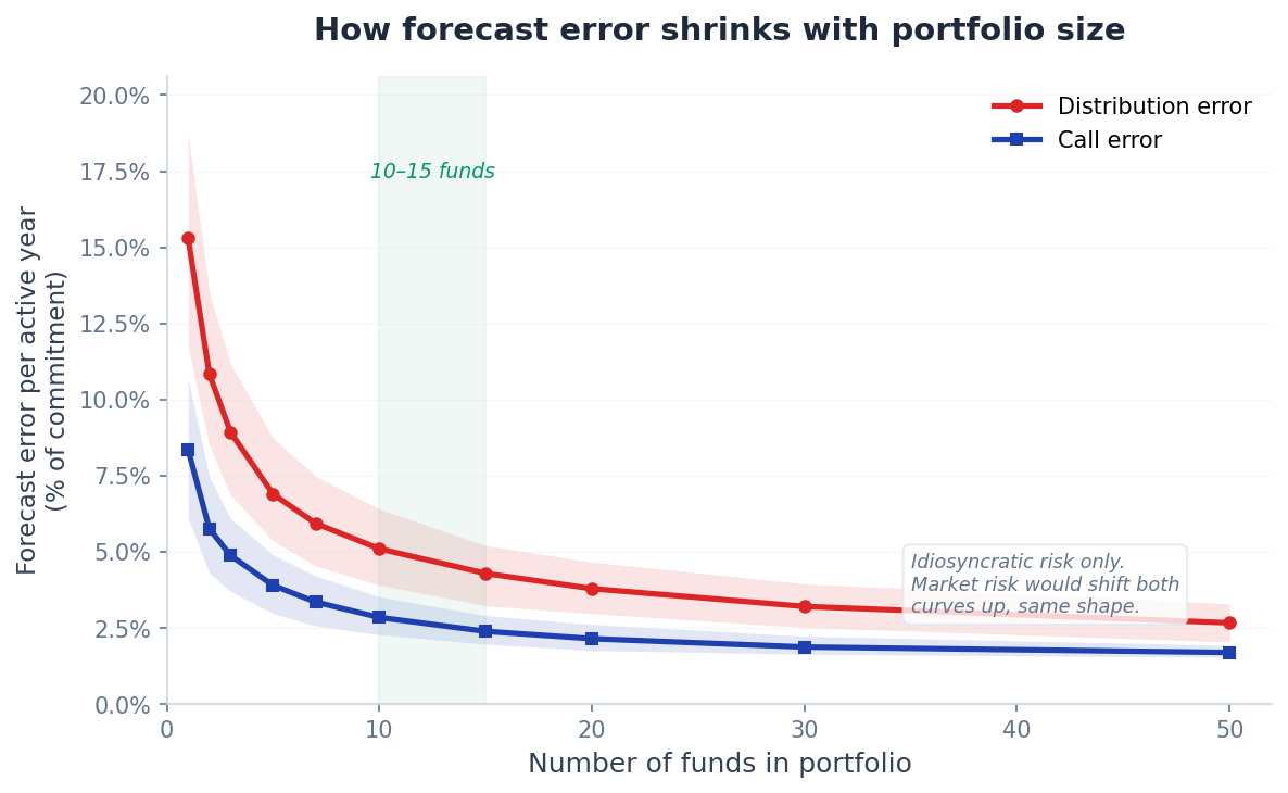
An important caveat: these numbers exclude market risk, the correlated shocks that hit all funds simultaneously (like the extended low-DPI environment since 2022). If we assumed, say, a 4% market risk floor, the 1-fund error would rise from 15% to ~19%, and the 10-fund error from 5% to ~9%. The error still drops substantially with diversification, but the percentage reduction is smaller (roughly 53% instead of 67%). The takeaway is the same: more funds help a lot, but don’t anchor on the precise reduction percentages. They depend on the level of market risk, which varies by vintage and macro environment.

What this looks like in practice

The chart below shows one simulated example. Each fund has a $1M commitment. The top row shows capital calls (years 1-5), the bottom row shows distributions (years 5-10). Blue bars are the forecast; red bars are what actually happened.

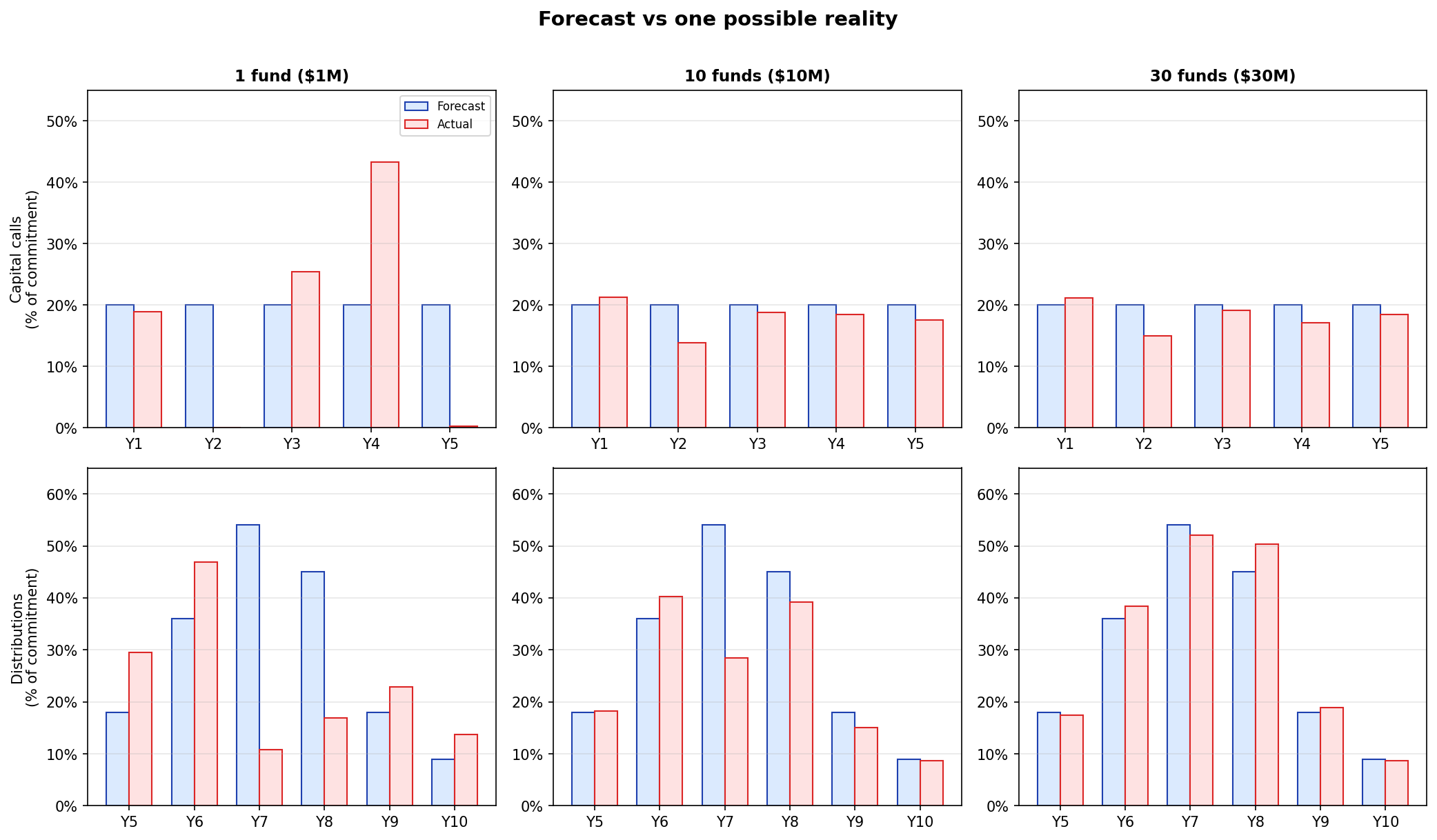
With one fund, both rows tell the same story: reality departs from the smooth forecast. This fund called nearly half its commitment in Year 4 alone, and returned only 1.4× instead of the forecast 1.8×. At 10 funds, the gaps narrow. At 30, the bars are closely aligned: most of the individual randomness has cancelled out.

A simplified model you can audit

We deliberately chose a simple model: the entire simulation is built in an Excel workbook where every formula is visible. Press F9 and all the random numbers regenerate, giving you a new scenario instantly. Download the Excel model.

A companion Python script automates the same formulas across 1,000 iterations to produce the charts above. Available on request.

Simple means assumptions. Some push the numbers in our favour, others against it. We tested multiple model variants, with different return distributions, lumpiness, and error metrics, and the specific numbers changed each time, but the pattern held: errors shrink as you add funds, with most of the benefit captured by 10-15.

Assumptions that overstate the benefit (reality might be weaker):

• ‍No market risk: our funds are modelled independently. In practice, funds share macro exposure. A downturn can delay exits across the board. This is the most important caveat: correlated risk raises the error floor for all portfolio sizes and reduces the percentage improvement from diversification (as illustrated above).
• ‍Equal commitments: every fund is $1M. Real portfolios concentrate in a few large funds, which reduces the effective diversification.
• ‍Uniform TVPI: we draw fund returns uniformly between 0.7× and 2.7×. In practice, PE returns are right-skewed: most funds cluster around 1.3-2.0× with a tail of outperformers. Less extreme dispersion means less cancellation across funds.

Assumptions that understate the benefit (reality likely stronger):

• ‍Same strategy: every fund is a PE buyout. Mixing in secondaries, venture, or infrastructure would create more timing diversity and more compensation.
• ‍Same vintage: all funds start in the same year. Real portfolios stagger vintages, so funds are at different life stages simultaneously: a 2018 fund in its distribution phase while a 2023 fund is still calling capital. This creates more independent variation in distributions across any given calendar year.
• ‍No lumpiness: we assume some distribution activity every year. Real exits are lumpier (some years nothing, some years a big exit), which would increase single-fund errors and make the diversification contrast sharper.

What this means for you

Don’t obsess over individual fund cash flow accuracy. Your single-fund forecast will be wrong. That’s the nature of PE cash flows. What matters is whether your aggregate forecast is directionally right. And it will be, once you have enough funds.

As of 10-15 funds, timing errors largely compensate. Distribution forecast error drops substantially compared to a single fund. Beyond 20, the improvement becomes marginal. If your portfolio is already in that range, you’re capturing most of the diversifiable benefit.

For market risk, diversify across assets and use scenarios. Fund-count diversification smooths timing errors but can’t protect against a market-wide distribution drought. That’s where strategy and vintage diversification help, and where running multiple scenarios, rather than relying on a single point estimate, becomes essential.

The bottom line: your cash flow models are more powerful than you think, as long as you have enough of them. The portfolio does the smoothing for you.